MS Excel: View hyperlink result at top of viewing area in Excel 2010

---

Also learn how to view a hyperlink result at the top of the viewing area in Excel 2010 | Excel 2007 | Excel 2003/XP/2000/97.

Question:  In Excel 2010, I have a worksheet that has the first 6 rows frozen. In the first 6 rows, I have hyperlinks to different cells in column B. When I click the hyperlinks, Excel tends to show the cell at the bottom of the viewing page.

I want the cell that the hyperlink refers to be displayed in the next row after the frozen rows. Can this be done?

Answer:  Let's take a look at an example.

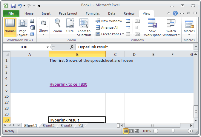
Below, we have an Excel spreadsheet with the first 6 rows hidden. In cell B5, we've created a hyperlink to cell B30. When we click on the hyperlink in cell B5, the spreadsheet looks as follows:

The hyperlink is at the bottom of the viewing area in the spreadsheet. We want to see row 30 directly under row 6.

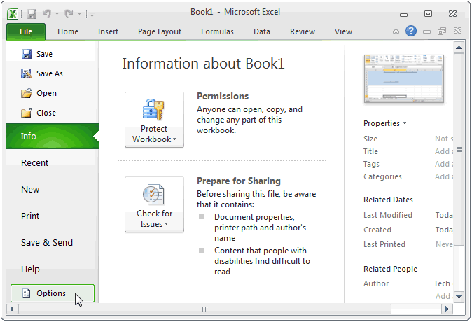
To fix this, select the File tab in the toolbar at the top of the screen and then click on Options at the bottom of the menu.

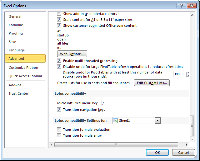
When the Excel Options window appears, click on the Advanced option on the left. Then scroll down to the Lotus Compatibility section in the right side of the window and select the checkbox called "Transition navigation keys". Click on the OK button.

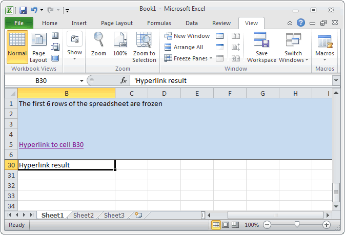
Now when you click on the hyperlink in cell B5, your spreadsheet should look as follows:

sumber : http://www.techonthenet.com